Expected hitting time estimates on finite graphs.
(Joint work with Laurent Saloff-Coste)$\global\def \R{\mathbb R}$ $\global\def \E{\mathbb E}$
Motivation: other connections
Hitting times are of interest in many probability-adjacent fields. Here are just a few examples:
economics & computer science: Understanding the running times of explore-exploit processes. If the explore process is a random walk, how long would it take to find somewhere we want to exploit?
physics: (Doyle, Snell 1984) Associate the random walk with an electric network: if we imagine the path taken by a single electron, then conductance ~ transition probability.
There are many papers written about estimating the effective resistances $\mathcal R (x \leftrightarrow y)$ on various graphs (frequently referred to as resistance problems).probability: Recent work (Dautenhahn, Saloff-Coste 2023) studies random walks on graphs that a "glued" together.
Here, it is important to know the hitting probabilities of where the graphs are glued.
Preliminaries
Our random process of interest is an
Under these assumptions, the random walks converges to a unique stationary measure $\pi$.
We are interested in the
Note that laziness (which implies aperiodicity) only contributes to a constant slow-down factor to $H(a,b).$
Related works:
(J. Cox 1989) Coalescing Random Walks and Voter Model Consensus Times on the Torus.
For $G = \Z_N^d$ and $a,b \in G$ such that
Proof in Cox '89 requires very good estimates for the eigenvectors and eigenvalues of $K$.
Markov Chains and Mixing Times (Levin, Peres 2017) provide a proof using effective resistance of the corresponding electric network, relying on the fact that the torus is vertex transitive.
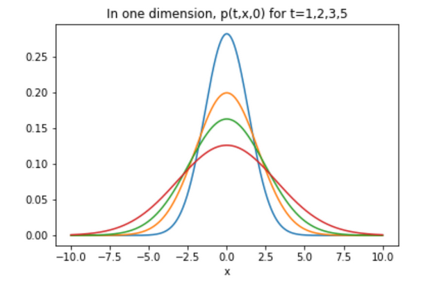
What is the heat kernel?
As the
With $y=0$, this is just the formula for a Gaussian with mean zero and variance $2 t$.
Heat kernels and $\theta$-Harnack graphs
(Grigor'yan, Saloff-Coste, Coulhon, Delmott, Barlow, etc.)These "lattice-like" graphs are those on which we have double-sided Gaussian bounds: $$ k^n(x,y) = \frac{K^n(x,y)}{\pi(y)} \asymp \frac{1}{V\left(x, n^{1/\theta}\right)} \exp \left(- \left( \frac{d(x, y)^\theta}{n}\right)^{\frac{1}{\theta-1}}\right), $$ for $\theta \geq 2$ and $V(x,r) = \sum_{y \in B(x,r)} \pi(y)$.
We will use the finite version of this definition.
Main result:
- $\theta$ is the walk-dimension of the graph
- $D$ is the diameter of the graph
- $V(x,r) = \sum_{y \in B(x,r)} \pi(y)$, where $B(x,r)$ is the ball of radius $r$ centered at $x$
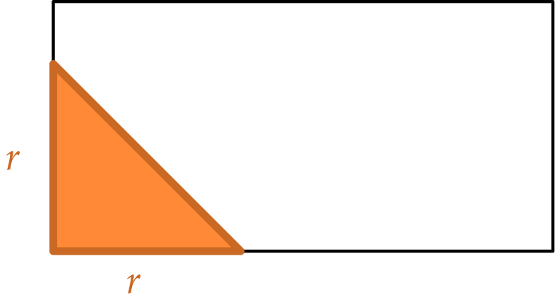
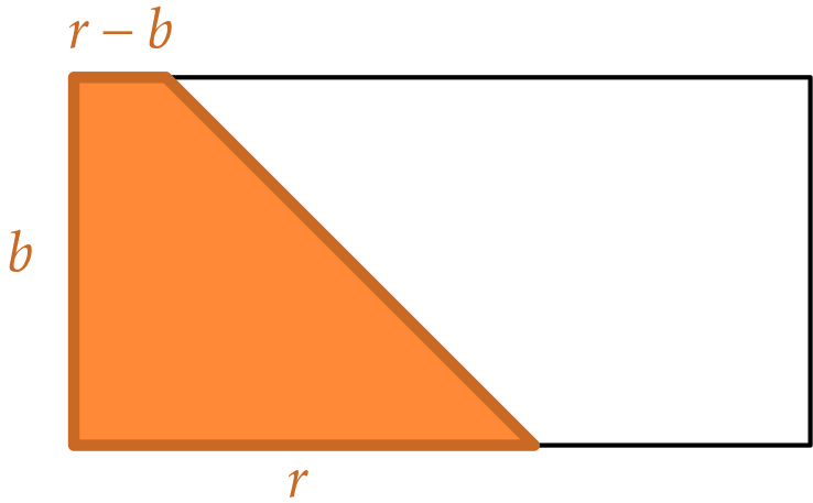
For lazy simple random walk on a regular graphs, $$H(a,b) \asymp |G| \sum\limits_{n=0}^{2D^\theta} \frac{1}{\#B(b,n^{1/\theta})}.$$
Example: Rectangular torus
Consider a rectangular $2$-dimensional torus, $G = \Z_a \times \Z_b$, where $a \geq b$.
This is a $2$-Harnack graph.
Let $x,y \in G$ be such that $d(x,y) \asymp D$.
Example: Rectangular torus
Consider a rectangular $2$-dimensional torus, $G = \Z_a \times \Z_b$, where $a \geq b$.
Let $x,y \in G$ be such that $d(x,y) \asymp D$. We computed that for the simple random walk:
Recall from (Cox '89) for $\Z_N$ and $\Z_N^2$, we know \[ H(x,y) \asymp \begin{cases} N^2 &\text{if } d=1 \\ N^2 \log N &\text{if } d=2 \end{cases}\]
In general: $N$-torus with uneven side lengths
Consider a simple random walk on the torus $$\Z_{a_1} \times \Z_{a_2} \times \cdots \times \Z_{a_N},$$ where $1 \leq a_1 \leq a_2 \leq \cdots \leq a_N.$ For two points $x,y$ such that $d(x,y) \asymp a_N$, $$H(x,y) \asymp_N \max \left\{ \prod_{i=1}^N a_i, a_N a_{N-1} \log \left(\frac{a_{N-1}}{a_{N-2}}\right), a_N^2\right\}.$$
Example: Birth-death chains
The state space is $\{0,1,\dotsc,N\}$ and transition probabilities can be specified by the information $\{(p_k, r_k, q_k)\}_{k=0}^N$. Consider a chain such that $\pi(k) \asymp (1 + k)^\alpha$.
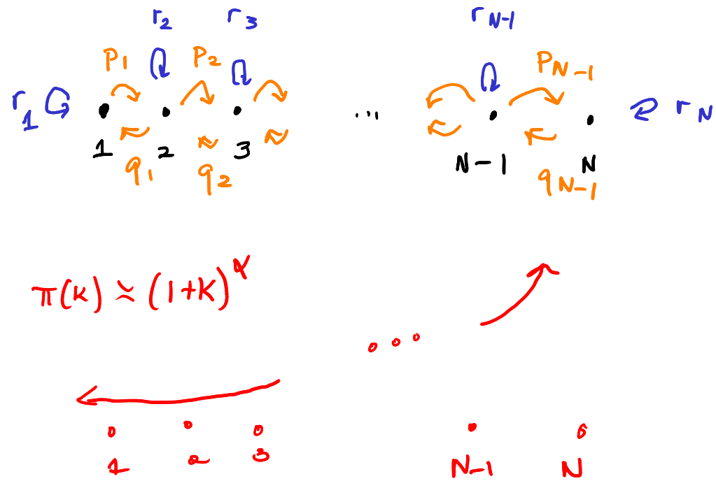
With a fixed $\pi$, it is straightforward to reverse engineer the transition probabilities so that the chain is reversible and converges to $\pi$. In our case, we expect $p_k$'s to be bigger than $q_k$'s.
\[ H(N,0) \asymp \begin{cases} N^{\alpha+1} &\text{if $\alpha>1$},\\ N^2 \log N &\text{if $\alpha = 1$},\\ N^2 &\text{if $0\le \alpha<1$}. \end{cases} \]
Example: Fractal graphs (Sierpinski Gasket)


In general, for Ahlfors-regular graphs
These are graphs where $\#B(y,r) \asymp r^\alpha$, which implies that $|G| \asymp D^\alpha$.
Using our theorem, we have that for $x,y$ such that $d(x,y) \asymp D$,
$$H(x,y) \asymp \begin{cases}
D^{\alpha} &\text{if $\alpha> \theta$},\\
D^\theta \log D &\text{if $\alpha = \theta$},\\
D^\theta &\text{if $0\le \alpha<\theta$}. \end{cases}$$
In the context of $\theta$-Harnack graphs, this behavior is analogous to the transition in $\Z^d$ from
The behavior at the transition can be more complex!
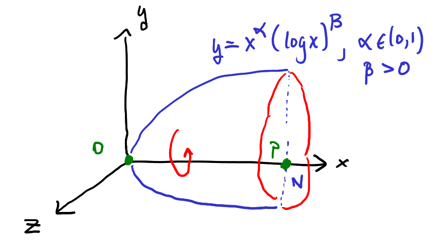
Fix $\alpha = 1/2$ and $\beta > 0$. The points $o = (0,0,0)$ and $p = (N,0,0)$ are roughly diameter apart. $$H(p,o) \asymp \sum_{n=0}^{N} \frac{1}{V(o,\sqrt{n})} \asymp \begin{cases} N^2(\log N)^{2\beta} &\text{if } \beta \in (1/2,+\infty) \\ N^{2} (\log N)(\log\log N) &\text{if } \beta = 1/2 \\ N^{2} \log N &\text{if } \beta \in (-\infty, 1/2). \end{cases} $$ In general, $H(x,y)$ can involve arbitrary slowly varying functions.
Proof sketch
The (normalized) discrete Green's function is a function $\mathcal G: G \times G \to \R$, where \[ \mathcal G (x,y) = \sum_{n = 0}^\infty (k^n(x,y) - 1), \] and $k^n(x,y) = K^n(x,y)/\pi(y)$.
Main Lemma: For all $x, y \in G$, \[H(x,y) = \mathcal G (y,y) - \mathcal G(x,y)\]
We first obtain bounds on the discrete Green's function using heat kernel bounds: $$ k^n(x,y) = \frac{K^n(x,y)}{\pi(y)} \asymp \frac{1}{V\left(x, n^{1/\theta}\right)} \exp \left(- \left( \frac{d(x, y)^\theta}{n}\right)^{\frac{1}{\theta-1}}\right), $$
When $d(x,y) = 0$, the exponential term disappears. There exists $C_1, C_2 > 0$ such that for all $x \in G$, \[ \mathcal G(x,x) \geq C_1 \sum_{0 \leq n \leq 2D^\theta} \frac{1}{V(x,n^{1/\theta})} - C_2 D^\theta. \]
When $n \geq D^\theta$, the volume term disappears and remaining exponential terms sum to a constant. When $d(x,y)^\theta \leq n \leq D^\theta$, the exponential term is bounded above by 1. For all $x,y \in V$, \[|\mathcal G(x,y)| \lesssim \sum_{d(x,y)^\theta \leq n \leq 2D^\theta} \frac{C}{V(x,n^{1/\theta})}\]
The last ingredient is a lower bound on $H(x,y)$: $H(x,y) \gtrsim D^\theta$ which we obtain by using exit time estimates.